This is the second of three posts focusing on the limitations of pre-aggregated metrics. The first one explained how, by pre-aggregating, your flexibility is tightly constrained when trying to explore data or debug problems. The third can be found here.

The nature of pre-aggregated time series is such that they all ultimately rely on the same general steps for storage: a multidimensional set of keys and values comes in the door, that individual logical “event” (say, an API request or a database operation) gets broken down into its constituent parts, and attributes are carefully sliced in order to increment discrete counters.

This aggregation step—this slicing and incrementing of discrete counters—not only reduces the granularity of your data, but also constrains your ability to separate signal from noise. The storage strategy of pre-aggregated metrics inherently rely on a countable number of well-known metrics; once your requirements cause that number to inflate, you’ve got some hard choices to make.

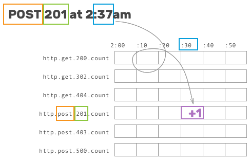
Let’s walk through an example. As in our previous post, given an inbound request to our API server, a reasonable metric to track might look something like this:

statsd.increment(`http.${method}.${status_code}.count`)

(A note: many modern time series offerings implement attributes like method and status_code as “tags,” which are stored separately from the metric name. They offer greater flexibility but the storage constraints are ultimately the same, so read on.)

Some nuts and bolts behind time series storage

To understand this next bit, let’s talk about how these increment calls map to work on disk. Pre-aggregated time series databases generally operate under the same principles: after defining a key name and a chosen granularity, events trigger writes to a specific bucket based on its attributes and the associated time.

This allows writes to be handled incredibly quickly, storage to be relatively cheap when the range of possible buckets is fairly small, and reads to be easily read sequentially.

The problem, then, is that the number of unique metrics directly affects the amount of storage needed to track all of the metrics—not the underlying data or traffic but the number of these predicted, well-defined parameters. As touched on above, there are two surefire ways to dramatically increase this number (and cause some serious stress on your time series storage):

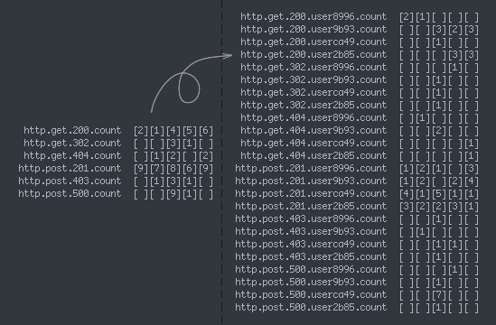
1. Each new attribute added to a set of metric names might increase the number of unique metrics exponentially, as the storage system has to track the cross product of each combination of values. You have to either accept that combinatorial explosion or choose to track only the first-order slice for a given attribute (just http.${hostname}.count).
2. Track an attribute with a particularly large set of potential values. Common high-cardinality attributes in this case are things like user ID, OS/SDK version, user agent, or referrer—and could cause the storage system to allocate a bucket for each discrete value. You have to either accept that storage cost or use a whitelist to only aggregate metrics for a set number of common (or important) user IDs/OS versions/user agents/etc.

A fabricated example illustrating both #1 and #2: adding a new attribute (user ID) to HTTP method + status code metrics causes the number of metrics to balloon—and this example only involves 4 distinct user IDs!

It’s painful for any service to be unable to think about metrics in terms of user segments, but crucial for any platform with a large number of distinct traffic patterns to do so. At Parse, for example, being able to identify a single app’s terrible queries as the culprit for some pathological Mongo behavior allowed us to quickly diagnose the problem and blacklist that traffic. Relying on pre-aggregated metrics would have required us to pick our top N most important customers to pay attention to, while essentially ignoring the rest.

Ultimately, no matter the specific pre-aggregated metrics tool, it’s all the same under the hood: constraints inherent in the storage strategy hobble you, the user, from being able to segment data in the most meaningful ways.

Curious to see how we’re different? Give us a shot!

Honeycomb can ingest anything described above, and do so much more. If you’re tired of being constrained by your tools—and you realize that there are some breakdowns in your data (user ID? application or project ID?) that you’ve always wanted but been conditioned to avoid—take a look at our long-tail dogfooding post to see this in action, or sign up and give us a try yourself!

Next, we’ll take a look at how, sometimes, simply being able to peek at a raw event can provide invaluable clues while tracking down hairy systems problems.

This is the first of three posts focusing on the limitations of pre-aggregated metrics, each corresponding to one of the “pre”, “aggregated”, and “metrics” parts of the phrase. The second can be found here.

Pre-aggregated, or write-time, metrics are efficient to store, fast to query, simple to understand… and almost always fall short of being able to answer new questions about your system. This is fine when you know the warning signs in your system, can predict those failure modes, and can track those canary-in-a-coal-mine metrics.

But as we level up as engineers, and our systems become more complicated, this stops being feasible: things are going to start breaking in unpredictable ways, and we need tools that can allow our future selves to be one step ahead of our past selves.

Let’s look at a situation in which this would be frustrating in the wild. Imagine we’re running a Cassandra cluster and want to monitor read and write latencies. (Really, any database might work here, Cassandra just exposes built-in metrics that suit our purposes nicely.)

Seems like a pretty reasonable assumption to start off with what the Cassandra folks decided to package up for us by default! We get to work, wire these metrics into a time series system, and we might end up with a few graphs like this, tracking the AVG by default and maybe the P95 if we’re feeling fancy:

Well, great! This seems fine, four graphs are pretty easy to keep an eye on. Except… sometimes we care whether a write is an increment vs an update vs a deletion! Or which column family/table we’re writing to. And averages are fine, but percentiles are better and sums illustrate total load on our system—so, soon enough, our four graphs now look a little more like:

… A little less straightforward to skim through, now.

By relying on pre-aggregation, we’ve lost the ability to get answers tailored to the question we’re asking (e.g. “Some of my database writes have been timing out, what’s going on?”); instead, we have to rely on answers that were packaged up for us in the past. We’re also necessarily biased by the graphs already in front of us, and can be blinded to other potential root causes.

Even given the above graphs, produced by storing just the first-order slices on the operation and table attributes, we’re unable to graph the cross product—for example, only updates affecting libdata—without first defining a new metric (db.op.updates.ns.libdata.latency.avg) and waiting for our graph to fill in with new data.

When each postmortem ends with an action item or three to add new metrics to a dashboard, the “anticipate everything; graph everything” strategy quickly enters a tailspin.

Intrigued? Give us a shot!

Honeycomb can produce any of the graphs shown above, and so much more. By preserving data for aggregation at query time, we can log whichever attributes tickle our fancy as a full event—then group by an arbitrary combination of those attributes or filter out all but an arbitrary slice of data.

Take a look at what Honeycomb’s approach looks like by browsing through our dogfooding posts, or just give us a whirl today!

Up next, we’ll talk a bit about the problem with the “aggregation” side of “pre-aggregation”—how implementation details of the aggregation step can make it next to impossible to get as deeply and flexibly into our data as we need.

Welcome! This will be a semi-regular series, where we answer frequently asked questions in short, digestible bites. Or if you prefer long philosophical essays about the future of observability, go here.

Ten short questions on getting started with Honeycomb

Ask your own questions! Find us as @honeycombio on twitter.

1. Is this a tool for ops and firefighting?

Yes! But not exclusively!

2. Is this a tool for instrumenting your application code?

Sure! But not exclusively! It’s for all these things and more, providing a familiar interface for all your ops, dev, and database needs.

3. Wait, is Honeycomb for developers or operations?

YES, all of those things! It’s a debugging power tool for anyone who needs to ask ad hoc, realtime queries about behavior or events.

4. How can I get data in?

Send JSON to our API, basically. We have lots of open-source wrappers and libs and tailers to get you started.

5. Is it super expensive?

Only if you want it to be. Pricing is based on retention and throughput. With good sampling hygiene, you can control costs at high volume.

6. Don’t you care about how many servers I have?

What’s a server? Just kidding, but no. Pay for what you use. We think the per-server model is archaic and broken.

7. This sounds a lot like Scuba, the Facebook internal observability tool.

Yup! Honeycomb has lots of Scuba DNA. We fell in love with the exploratory model at Facebook, and based early mocks off the whitepaper.

8. This sounds a lot like Splunk, SignalFX, NewRelic, Librato, DataDog, Graphite, ELK, Wavefront, Papertrail, Druid, Prometheus, InfluxDB…

Haha. Well, we’re all using similar words – “realtime”, “exploratory”, “interactive”. But we’re very different. Schedule a demo!

9. Can I play with it somewhere, before importing my own data?

Definitely. We have demo data sets you can play with to see how things work. Just sign up and drop us a line to see our streaming samples.

10. Sorry, I have the attention span of a gnat … how do I ask a question?

Email us at support@honeycomb.io, or tweet to us at @honeycombio on twitter – we’ll respond there and post it here, too!

Today we’re open sourcing our SDK for Ruby, so you can gain the same sort of insight into the behavior of your Ruby apps & services as people are already experiencing with Go, Python, and Javascript.

Install the Gem

The library is available from rubygems. To get started, add this line to your Gemfile:

gem "libhoney", "~> 1.0"

If you’d rather track the bleeding edge, you can reference our git repo directly:

gem "libhoney", :git => "https://github.com/honeycombio/libhoney-rb.git"

API Structure

The Ruby API shares the same basic structure of our other SDKs, with objects representing:

1. An instance of the library (in the Ruby SDK this is spelled Libhoney::Client)
2. Events that are sent to honeycomb
3. Builders for generating events that share common fields
4. Responses

Initializing the library

To get an instance of Libhoney::Client:

require 'libhoney'
...

libhoney = Libhoney::Client.new(:writekey => "my_writekey",
                                :dataset => "my_dataset")

Sending events

ev = libhoney.event # create an event object
ev.add_field("response_time_ms", 0.5) # add a single field/value
ev.add({ field1 => val1,
         field2 => val2 }) # add multiple fields/values at once
ev.sample_rate = 5 # optionally set the sample rate
ev.send

# the event methods are chainable, so you can also do:
libhoney.event
  .add({ field1 => val1,
         field2 => val2})
  .send

Using builders

You can use a builder to create many similar events as follows:

# create a builder for fields that will be shared
builder = libhoney.builder
builder.add_field("session_id", "012345abcdef")

# then any event created from this builder will inherit the session_id field
builder.event
  .add_field("database_ms", 0.5)
  .send
builder.event
  .add_field("external_service_roundtrip_status", 500)
  .send

The Libhoney::Client instance also acts as a builder. Builders can be created from other builders, with fields being inherited along the way:

# add a field to the libhoney builder
libhoney.add_field("user_agent", "Mozilla/5.0 ...")

# create a sub-builder from libhoney, which will inherit the user_agent field
builder = libhoney.builder("session_id", "012345abdef")

# so this event will contain 3 fields (user_agent, session_id, database_ms)
builder.event
  .add_field("database_ms", 0.5)
  .send

Responses

You can optionally subscribe to responses for all events sent through our API:

# on a separate thread from the part of the app sending events
resps = libhoney.responses

loop do
  resp = resps.pop()
  break if resp == nil
  puts "sending event with metadata #{resp.metadata} took 
    #{resp.duration}ms and got response code #{resp.status_code}"
end

You can also associate metadata with an individual event and it will be communicated back through the response object:

ev = builder.event
ev.metadata = 42 # can be anything, a string, a hash, etc
ev.send

response = libhoney.responses.pop()
puts response.metadata # => 42

That’s it!

For API documentation, visit rubydoc.info. For higher level documentation, head to our docs.